Part 1 - Correlation and Causation
I've been looking at regressions and trying to understand how much I should trust regressions. There are a few questions I'm keen to look at:
Why is regression an
When regression is an appropriate technique, but there are many other variables, how successful can controlling for confoungers be, and how comprehensive must this adjustment be?
When it works tolerably, but not perfectly, how far away from the 'true' value does it fall, and how does this change with varialbes such as the number of confounders controlled for, the complexity of the situation, the degree of non-linearity etc.
The set up
To investigate this, I first set up the ability to make random graphs:
# Setting up the dataclasses used to define graphs
@dataclass

class Point:

    point_id: int

    x: int

    y: int

    parents: list

    children: list

    error: float

    value: float = 0


@dataclass

class Link:

    point: Point

    strength: float


@dataclass

class Graph:

    points: List[Point]
The graph is richer than necessary but it helps make operations more flexible on the graph.
We can then define different graphs to model situations of varying complexities.
def build_simple_regression(n_inputs: int):
        # adds the output node

        points = [Point(

            x=50,

            y=50,

            parents=[],

            children=[],

            point_id=n_inputs - 1,

            error=random.uniform(0, 1)

        )]


        # adds the input nodes at the beginning of the points list

        for i in range(n_inputs - 1):

            conx_str = random.normalvariate(0, 1)

            points.insert(-1, Point(x=50 + (i - (n_inputs / 2)) * 10,

                                    y=20,

                                    parents=[],

                                    children=[Link(points[-1], conx_str)],

                                    point_id=i,

                                    error=random.uniform(0, 1)))

            points[-1].parents.append(Link(points[i], conx_str))


        return Graph(points)
def build_random_diagonal(n_nodes: int, density: float):
        scale = 100  # just for graphing, has no material impact


        # add n_nodes points randomly

        points = []

        for i in range(n_nodes):

            points.append(Point(x=random.randrange(scale),

                                y=random.randrange(scale),

                                parents=[],

                                children=[],

                                point_id=i,

                                error=random.uniform(0, 1)))


        # sort points from bottom-left to top-right

        points.sort(key=lambda p: math.hypot(p.x, p.y))


        # connect points by density, with direction from bottom-left to top-right

        for n1, p1 in enumerate(points):

            p1.point_id = n1

            for n2, p2 in enumerate(points[:n1]):

                distance = math.hypot(p1.x - p2.x, p1.y - p2.y)

                if distance < scale * density:

                    conx_str = random.uniform(-1, 1)

                    p1.parents.append(Link(p2, conx_str))

                    p2.children.append(Link(p1, conx_str))


        return Graph(points)
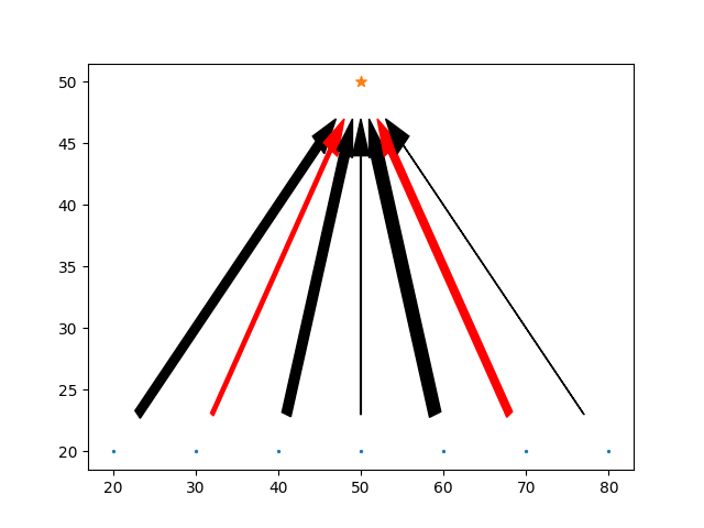
It's useful to plot these causal graphs to understand them. Arrow widths indicate the (linear) connection strength, red arrows indicating negative connections, and a star indicating the final, output variable. this variable is no different to any other in principle, but it designed to have not outgoing connections, and will be the target of all simulated regressions.
def plot_directed_graph(graph: Graph):
    # add a point on the graph for each point

    plt.scatter([p.x for p in graph.points[:-1]], [p.y for p in graph.points[:-1]], s=2)

    plt.scatter(graph.points[-1].x, graph.points[-1].y, s=50, marker="*")


    # add arrow from parent to child to show the directed graph

    for p1 in graph.points:

        for l in p1.children:

            color = 'red' if l.strength < 0 else 'black'

            gap_x = l.point.x - p1.x

            gap_y = l.point.y - p1.y

            plt.arrow(x=p1.x + 0.1 * gap_x,

                      y=p1.y + 0.1 * gap_y,

                      dx=(l.point.x - p1.x) * 0.8,

                      dy=(l.point.y - p1.y) * 0.8,

                      head_width=2,

                      length_includes_head=True,

                      width=l.strength * 0.7,

                      color=color)


    plt.show()
Before we look at whether controlling for confounders works, we first need to be clear about what we're actually trying to do. The ideal of a causal graph in this kind of form is following the tradition of structured equation modelling. The idea, following Pearl, of the true causal impact is to take one node, and make some change to it, and then allowing this change to propagate through the graph.
Since we're initially dealing with simple linear models with no loops, we can understand the impact of a variable a on a second variable b by tracing all of the paths from a to b, for each path find the product of all the weights on the path, and then sum the impact via each path.
A more experimental approach is also possible, by making small changes to the input variable and assessing the impact on the final variable. With these linear models only two points are needed to find the impact but this approach should generalize to much more complex models.
Method A - summing paths:
def forward_causal_impact(graph: Graph, selected_var: int = 0, seed: int = 0, final_var: int = 0):
    # takes each point and assigns it a value based on the value of its predecessors, the connection strengths,

    # and the size of the error.

    # requires that the points form a directed acyclic graph ordered such that a parent precedes all of its children

    if not final_var:

        final_var = len(graph.points) - 1


    deltas = list(np.arange(-1, 1, 0.1))

    finals = []


    for delta in deltas:

        np.random.seed(seed)

        selected_point = graph.points[selected_var]

        assert selected_point.point_id < len(graph.points)


        for p in graph.points:

            p.value = 0


        for p in graph.points:

            p.value = sum([link.strength * link.point.value for link in p.parents]) + np.random.normal(0, p.error)

            if p.point_id == selected_var:

                p.value += delta


            if p.value > 1000:

                print([(link.strength, link.point.value) for link in p.parents], p.error)


        finals.append(graph.points[final_var].value)


    deltas_input = np.array(deltas)

    deltas_input = deltas_input.reshape(-1, 1)

    finals_input = np.array(finals)

    regr = LinearRegression().fit(deltas_input, finals_input)

    impact = regr.coef_[0]    # regression unnecessary for linear models but important for sensitive, non-linear cases

    return deltas, finals, impact
Method B - testing interventions:
def get_causal_impact(graph: Graph, selected_var: int, final_var: int):
    selected_point = graph.points[selected_var]

    assert selected_point.point_id == selected_var

    downstream = reachable(selected_var, graph)

    upstream = reachable(final_var, graph, reverse=True)

    midpoints = [p1 and p2 for p1, p2 in zip(downstream, upstream)]

    midpoints[final_var] = 1

    # print(midpoints)

    traversed = [0] * len(graph.points)

    traversed[selected_var] = 1

    impacts = [0] * len(graph.points)

    impacts[selected_var] = 1

    for n, p in enumerate(graph.points):

        if not midpoints[n]:

            continue

        # this checks that all of the parents have been traversed

        # if they have then their impact values are set, and so the impact value of the child can be calculated

        impacts[n] = sum([x.strength * impacts[x.point.point_id] for x in p.parents])


    # plot_directed_graph_paths(graph, source=selected_var, labels=impacts)

    return impacts
These models should and do return the same values, for both the simple and complex graph types as generated above, giving confidence in this as a measure of the impact.
We can now go about simulating regressions, and test under what conditions, a regression successfully identifies the causal impact of the variables.
We need the ability to run regression tests
def test_subset(outcome_data, selected_var, n_confounds=5):
    # outcome_data has shape (n_trials, n_nodes)

    dependent_var = outcome_data[:, -1]

    independent_var = outcome_data[:, selected_var]


    # puts the selected variable first as a column vector, and then adds the chosen number of confounders

    if n_confounds > outcome_data.shape[1] - 2:

        confounds = np.concatenate((outcome_data[:, :selected_var], outcome_data[:, selected_var + 1:-1]), axis=1)

    elif n_confounds == 0:

        confounds = None

    else:

        # sample confounders randomly from n_nodes except the final node and selected var

        var_range = list(range(outcome_data.shape[1] - 1))

        var_range.remove(selected_var)

        confounds_xs = random.sample(var_range, k=n_confounds)

        confounds = outcome_data[:, confounds_xs]


    if n_confounds:

        X = np.insert(confounds, 0, independent_var, axis=1)

    else:

        # X must be a 2D array to feed into the LinearRegression

        X = independent_var.reshape((len(independent_var), -1))


    regr = LinearRegression().fit(X, dependent_var)

    return regr.coef_[0]
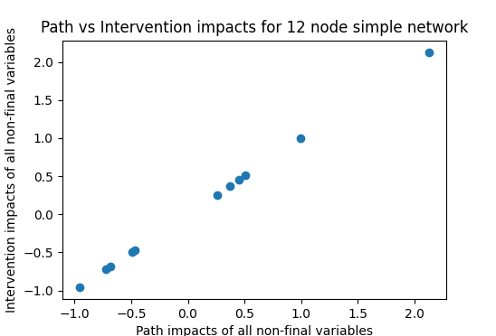
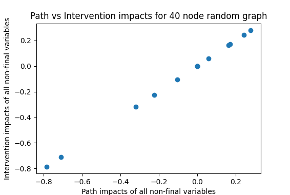
Now we can check how well these three methods agree on the impact of one variable. Comparing the summing-paths method and testing interventions,
Path and intervention approaches, confirming equivalence
We can then check whether a fully-adjusted regression (including all variables in the regression) also matches these results:
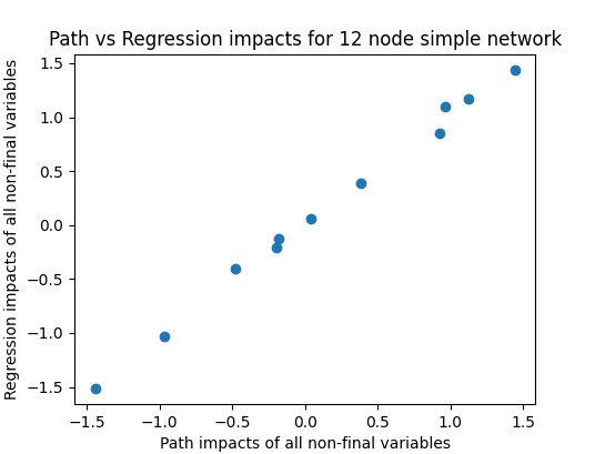
Ah..
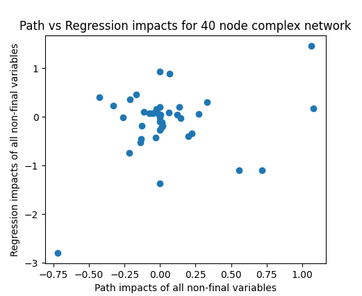
With the simple causal network this is working well, with only small deviations as to be expected with a random trial (sample of 200 used here). Not so for the random network where there seems to be hardly a correlation between the two in this example, and this is borne out by repeated runs. Running 50 trials here yields an average correlation of 0.356, showing that the fully-controlled impact explains hardly more than 10% of the variance in the true causal impact.
If we remove variability by pushing the number of trials in the regression from 200 up to 2000 and 20000, we get correlations of 0.409 and 0.55 respectively. With 200,000 trials, the correlation goes up to 0.644. This jump in the corrlation is surprising to me. I think what is happening here is that all variables whose impact on the final variable is only through intermediate nodes, then the regression, when including all nodes, will go to zero at the limit, but at sample sizes of 200 and even 2000, there is still significant noise in the estimates of these parameters. For example, here is one run with 200,000 trials that produces a correlation of 0.884.
This is in line with the theoretical expectation that if we have a regression of the form \(y = b0 + b1\) then